Bloom Filters: Probabilistic Data Structures for Fast Set Membership Testing in Go

Table of Contents

Working with large-scale data at Semrush, I’ve often faced the classic problem: “Is this item in my massive dataset?” When you’re dealing with billions of entries, even the most optimized database queries can become a bottleneck. That’s where Bloom filters come in - a probabilistic data structure that changed how I think about membership testing.

The data structure was proposed by Burton Bloom in a 1970 paper titled “Space/Time Trade-offs in Hash Coding with Allowable Errors”. Yes, 1970! Sometimes the old solutions are still the best ones.

Why Bloom Filters Matter #

Picture this scenario: you have data stored across multiple files or database shards, and you need to check if a certain key exists. Reading from disk is expensive - we’re talking milliseconds in the best case. A Bloom filter acts as a lightning-fast cache with interesting probabilistic properties:

If the filter says the key is not present, it’s 100% certain - no need to check the actual storage
If the filter says the key is present, there’s a small chance it’s lying (false positive)

In my experience, when most queries return “not found” (which is surprisingly common in real systems), Bloom filters can reduce disk access by 95% or more. The probabilistic nature might sound like a weakness, but it’s actually what enables the incredible speed and space efficiency.

As Bloom himself put it:

The new hash-coding methods to be introduced are suggested for applications in which the great majority of messages to be tested will not belong to the given set. For these applications, it is appropriate to consider as a unit of time (called reject time) the average time required to classify a test message as a nonmember of the given set.

How Bloom Filters Work #

A Bloom filter is essentially a clever variation of a hash table with open addressing. At its core, it’s just an array of bits (size m) and some number (k) of hash functions. Each hash function maps arbitrary data to an integer in the range [0, m-1].

The filter supports two operations:

Insert an item: Hash the item with all k hash functions and set the corresponding bits to 1. Simple as that.

Test membership: Hash the item with all k hash functions. If any bit is 0, return “false” with certainty. If all bits are 1, return “true” - but remember, there’s a small false positive chance.

Here’s how Bloom described it in the original paper:

The hash area is considered as N individual addressable bits, with addresses 0 through N - 1. It is assumed that all bits in the hash area are first set to 0.

Next, each message in the set to be stored is hash coded into a number of distinct bit addresses, say a1, a2, . . . , ad. Finally, all d bits addressed by a1 through ad are set to 1.

To test a new message a sequence of d bit addresses, say a'1, a'2, … a’d, is generated in the same manner as for storing a message. If all d bits are 1, the new message is accepted. If any of these bits is zero, the message is rejected.

Let me show you a visual example:

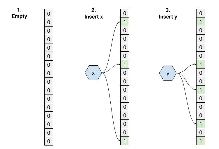
We start with an empty bloom filter with m=16 and k=3. All bits initialized to 0.
Insert “x”. The three hashes return indices 1, 6, 15, so we set those bits to 1.
Insert “y”. Hashing gives us 6, 9, and 13. Note that bit 6 overlaps with “x” - that’s totally fine and expected.

Now for membership testing:

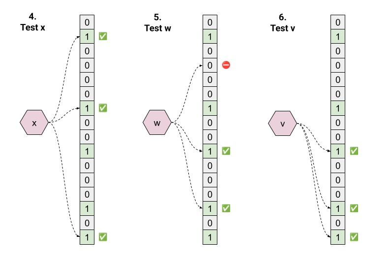
Test “x”. Hashing returns 1, 6, 15; all these bits are 1, so we return “true”. This is a true positive.
Test “w”. Hashing returns 3, 9, 13. Bit 3 is 0, so we return “false” with certainty.
Test “v”. Hashing returns 9, 13, 15; all these bits are 1, so we return “true”. But “v” was never inserted - this is a false positive!

The beauty is in the simplicity. By the law of contraposition, we can prove that all “false” answers are guaranteed to be true negatives.

Implementation in Go #

Here’s a clean implementation I’ve been using in production (well, a simplified version):

 1
 2
 3
 4
 5
 6
 7
 8
 9
10
11
12
13
14
15
16
17
18
19
20
21
22
23
24
25
26
27
28
29
30
31
32
33
34
35
36
37
38
39
40
41
42
43
44
45
46
47


// New creates a new BloomFilter with capacity m, using k hash functions.
// You can calculate m and k from the number of elements you expect the
// filter to hold and the desired error rate using CalculateParams.
func New(m uint64, k uint64) *BloomFilter {
  return &BloomFilter{
    m:      m,
    k:      k,
    bitset: newBitset(m),
    seed1:  maphash.MakeSeed(),
    seed2:  maphash.MakeSeed(),
  }
}

type BloomFilter struct {
  m      uint64
  k      uint64
  bitset []uint64

  // seeds for the double hashing scheme.
  seed1, seed2 maphash.Seed
}

// Insert a data item into the bloom filter.
func (bf *BloomFilter) Insert(data []byte) {
  h1 := maphash.Bytes(bf.seed1, data)
  h2 := maphash.Bytes(bf.seed2, data)
  for i := range bf.k {
    loc := (h1 + i*h2) % bf.m
    bitsetSet(bf.bitset, loc)
  }
}

// Test if the given data item is in the bloom filter. If Test returns false,
// it's guaranteed that data was never added to the filter. If it returns true,
// there's an eps probability of this being a false positive. eps depends on
// the parameters the filter was created with (see CalculateParams).
func (bf *BloomFilter) Test(data []byte) bool {
  h1 := maphash.Bytes(bf.seed1, data)
  h2 := maphash.Bytes(bf.seed2, data)
  for i := range bf.k {
    loc := (h1 + i*h2) % bf.m
    if !bitsetTest(bf.bitset, loc) {
      return false
    }
  }
  return true
}

This implementation uses double hashing - a neat trick to generate k different hash functions from just two base hashes. Much more efficient than computing k independent hashes.

The CalculateParams function helps you size your filter correctly:

 1
 2
 3
 4
 5
 6
 7
 8
 9
10
11
12
13


// CalculateParams calculates optimal parameters for a Bloom filter that's
// intended to contain n elements with error (false positive) rate eps.
func CalculateParams(n uint64, eps float64) (m uint64, k uint64) {
  // The formulae we derived are:
  // (m/n) = -ln(eps)/(ln(2)*ln(2))
  // k = (m/n)ln(2)

  ln2 := math.Log(2)
  mdivn := -math.Log(eps) / (ln2 * ln2)
  m = uint64(math.Ceil(float64(n) * mdivn))
  k = uint64(math.Ceil(mdivn * ln2))
  return
}

Check the math appendix if you want to understand where these formulas come from - it’s actually quite elegant.

Real-World Performance #

Let’s talk numbers. Say you want to store about 1 billion items with a 1% false positive rate (meaning 99% confidence when the filter says “yes”). Here’s what you get:

1

CalculateParams(1000000000, 0.01) ===> (9585058378, 7)

This means:

m ≈ 9.6 billion bits ≈ 1.19 GB of memory
k = 7 hash functions

Think about that - you can test membership for a billion items of arbitrary size using just 1.19 GB of RAM. The lookup is deterministic: exactly 7 hash computations, regardless of how many items are actually stored.

On my development machine, I’m seeing about 85 nanoseconds per lookup with this Go implementation. And this is without any serious optimization - I’m sure we could squeeze out another 2x with a faster hash function or SIMD instructions.

Compare that to even the fastest database lookup. Just the system call to read from an SSD would take microseconds - that’s 100x slower, and we haven’t even parsed the data yet.

Practical Applications #

At my previous job, we used Bloom filters extensively for:

Database query optimization: Before hitting the database to check if a user exists, check the Bloom filter first. Saved us countless unnecessary queries.
Distributed caching: Each node maintains a Bloom filter of its cache contents. Before requesting data from a peer, check if they likely have it.
Duplicate detection: In our data pipeline, we needed to detect duplicate events. A Bloom filter per time window worked perfectly.
Crawler URL filtering: When crawling websites, quickly check if we’ve seen a URL before without maintaining a massive set in memory.

Remember, Bloom filters shine when “the great majority of messages to be tested will not belong to the given set”. In my experience, this describes most real-world scenarios surprisingly well. Even with a 1% false positive rate, you’re only doing unnecessary work 1% of the time when the item exists - a fantastic tradeoff.

The Math Behind Bloom Filters #

Let’s understand why this works. Notation reminder:

m: size (in bits) of the filter
n: number of inserted keys
k: number of hash functions

For a specific bit, assuming uniform hash distribution, the probability it’s not set by a specific hash is:

$$p_0=1-\frac{1}{m}$$

The probability it’s not set by any of our k hash functions:

$$p_0=\left ( 1-\frac{1}{m}\right )^k=\left( \left ( 1-\frac{1}{m}\right )^m\right)^\frac{k}{m}$$

For large m, we can use the approximation $\lim_{m \to \infty}(1-\frac{1}{m})^m = e^{-1}$:

$$p_0\approx e^{-\frac{k}{m}}$$

After inserting n elements:

$$p_0\approx e^{-\frac{kn}{m}}$$

So the probability of a bit being 1 is:

$$p_1\approx 1-e^{-\frac{kn}{m}}$$

The false positive rate (probability all k hashes hit 1s for a new element):

$$p_{fp}\approx\left ( 1-e^{-\frac{kn}{m}} \right )^k\approx \varepsilon$$

To minimize this error rate, we differentiate with respect to k and find:

$$k_{optimal}= \frac{m}{n}\cdot \ln(2)$$

For example, with 1 million bits and 100,000 elements:

$$k= 10\cdot \ln(2)= 6.93 \approx 7$$

Working backwards from a desired error rate:

$$\frac{m}{n}\approx -\frac{\ln \varepsilon}{\ln^2(2)}$$

Want 1% false positive rate? You need:

$$\frac{m}{n}\approx -\frac{\ln 0.01}{\ln^2 (2)}=9.58$$

So about 9.58 bits per element. For 100,000 elements, allocate at least 958,000 bits and use 7 hash functions.

When to Use Bloom Filters #

After years of using them, here’s my advice:

Use Bloom filters when:

Most lookups are negative (item not in set)
False positives are acceptable but false negatives aren’t
You need consistent, fast performance
Memory is limited relative to dataset size

Don’t use them when:

You need to delete items (standard Bloom filters don’t support deletion)
You need exact membership testing
Your dataset is small enough to fit in a regular hash table
Positive lookups are more common than negative ones

There are variants like Counting Bloom Filters that support deletion, and Cuckoo Filters that offer better performance in some scenarios. But the classic Bloom filter remains my go-to for most use cases.

Conclusion #

Bloom filters are one of those beautiful computer science concepts that are both theoretically elegant and practically useful. They turn the apparent weakness of allowing false positives into a strength, achieving incredible space and time efficiency.

Next time you’re building a system that needs fast membership testing for large datasets, consider a Bloom filter. That 85-nanosecond lookup might just be what makes your system fly.

Complete Implementation #

Here’s the full code including the bitset helper functions:

  1
  2
  3
  4
  5
  6
  7
  8
  9
 10
 11
 12
 13
 14
 15
 16
 17
 18
 19
 20
 21
 22
 23
 24
 25
 26
 27
 28
 29
 30
 31
 32
 33
 34
 35
 36
 37
 38
 39
 40
 41
 42
 43
 44
 45
 46
 47
 48
 49
 50
 51
 52
 53
 54
 55
 56
 57
 58
 59
 60
 61
 62
 63
 64
 65
 66
 67
 68
 69
 70
 71
 72
 73
 74
 75
 76
 77
 78
 79
 80
 81
 82
 83
 84
 85
 86
 87
 88
 89
 90
 91
 92
 93
 94
 95
 96
 97
 98
 99
100


package bloom

import (
    "hash/maphash"
    "math"
)

// BloomFilter represents a Bloom filter data structure
type BloomFilter struct {
    m      uint64
    k      uint64
    bitset []uint64
    
    // seeds for the double hashing scheme
    seed1, seed2 maphash.Seed
}

// New creates a new BloomFilter with capacity m, using k hash functions.
func New(m uint64, k uint64) *BloomFilter {
    return &BloomFilter{
        m:      m,
        k:      k,
        bitset: newBitset(m),
        seed1:  maphash.MakeSeed(),
        seed2:  maphash.MakeSeed(),
    }
}

// Insert a data item into the bloom filter.
func (bf *BloomFilter) Insert(data []byte) {
    h1 := maphash.Bytes(bf.seed1, data)
    h2 := maphash.Bytes(bf.seed2, data)
    for i := range bf.k {
        loc := (h1 + i*h2) % bf.m
        bitsetSet(bf.bitset, loc)
    }
}

// Test if the given data item is in the bloom filter.
func (bf *BloomFilter) Test(data []byte) bool {
    h1 := maphash.Bytes(bf.seed1, data)
    h2 := maphash.Bytes(bf.seed2, data)
    for i := range bf.k {
        loc := (h1 + i*h2) % bf.m
        if !bitsetTest(bf.bitset, loc) {
            return false
        }
    }
    return true
}

// CalculateParams calculates optimal parameters for a Bloom filter
func CalculateParams(n uint64, eps float64) (m uint64, k uint64) {
    ln2 := math.Log(2)
    mdivn := -math.Log(eps) / (ln2 * ln2)
    m = uint64(math.Ceil(float64(n) * mdivn))
    k = uint64(math.Ceil(mdivn * ln2))
    return
}

// Bitset helper functions

// newBitset creates a new bitset with m bits
func newBitset(m uint64) []uint64 {
    // We need ceil(m/64) uint64s to store m bits
    size := (m + 63) / 64
    return make([]uint64, size)
}

// bitsetSet sets the bit at position pos to 1
func bitsetSet(bitset []uint64, pos uint64) {
    wordIndex := pos / 64
    bitIndex := pos % 64
    bitset[wordIndex] |= (1 << bitIndex)
}

// bitsetTest returns true if the bit at position pos is 1
func bitsetTest(bitset []uint64, pos uint64) bool {
    wordIndex := pos / 64
    bitIndex := pos % 64
    return (bitset[wordIndex] & (1 << bitIndex)) != 0
}

// Example usage:
func Example() {
    // Create a Bloom filter for 1 million items with 1% error rate
    m, k := CalculateParams(1000000, 0.01)
    bf := New(m, k)
    
    // Insert some data
    bf.Insert([]byte("hello"))
    bf.Insert([]byte("world"))
    bf.Insert([]byte("golang"))
    
    // Test membership
    exists := bf.Test([]byte("hello"))   // true
    exists = bf.Test([]byte("world"))    // true  
    exists = bf.Test([]byte("foo"))      // false (probably)
    exists = bf.Test([]byte("bar"))      // false (probably)
}

The bitset operations are straightforward bit manipulation - we pack 64 bits into each uint64 for efficiency. Writing your own implementation is surprisingly satisfying and you’ll understand the structure much better.

Have you used Bloom filters in production? What interesting applications have you found? I’m always curious to hear about creative uses of probabilistic data structures.